Measuring the performance of algorithms

In our previous article, Big-O notation and complexity theory, we saw how an algorithm categorized as \(O(n)\) is more efficient than one classified with a complexity of \( O(n^2)\). Still, we only compared the algorithms in theory. In this article, we will see how well the theory matches the practice by measuring the execution time of the two algorithms we saw in the previous article.

Measuring get_max_value

First, we will measure how long it takes to execute the code for the get_max_value algorithm. The code for this algorithm is the following.

After executing the above code and measuring the time to find the max value of five lists with 1000, 2500, 5000, 7500, and 10000 numbers, we will get a graph that looks like the following.

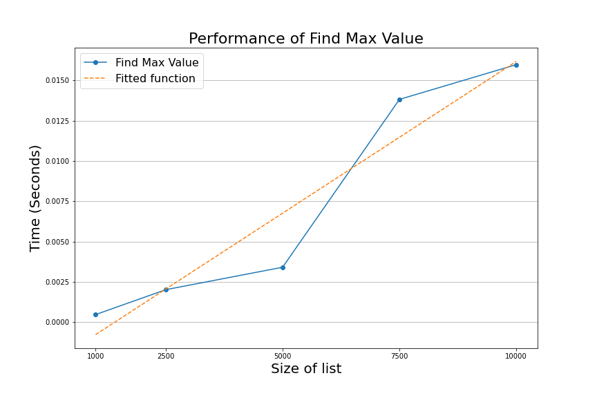
The blue line in the graph is the time in seconds it took for the algorithm to find the maximum number in each of the five lists, and the orange line is the average of all the runs.

We don't get an exact line when we graph the execution time. Instead, the execution time fluctuates as the algorithm processes the lists. However, we can see that, on average, our algorithm scales linearly. In other words, as the lists get larger, the time it takes for the algorithm to finish increases following a line pattern.

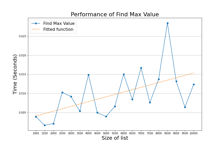
If we were to add more lists to our execution, we would see the same behavior.

Many factors contribute to the performance of algorithms in the real world. For example, computers execute many other processes in the background, which means that computer resources are shared between programs, impacting the time we measure.

This resource sharing means that we can get different measurements every time we run the algorithm, so the time we measure depends on the machine where the algorithm is executing.

For this reason, complexity theory focuses on counting the algorithm's computational steps. It is a machine-independent measure that is easy to relate to actual performance.

Measuring the bubble sort algorithm

Let's now take a look at the performance of our bubble sort algorithm.

We know that the bubble sort algorithm is \( O(n^2) \), and when we run the algorithm with the same list of numbers we used when running the get_max_value algorithm, we get a graph that looks like the following.

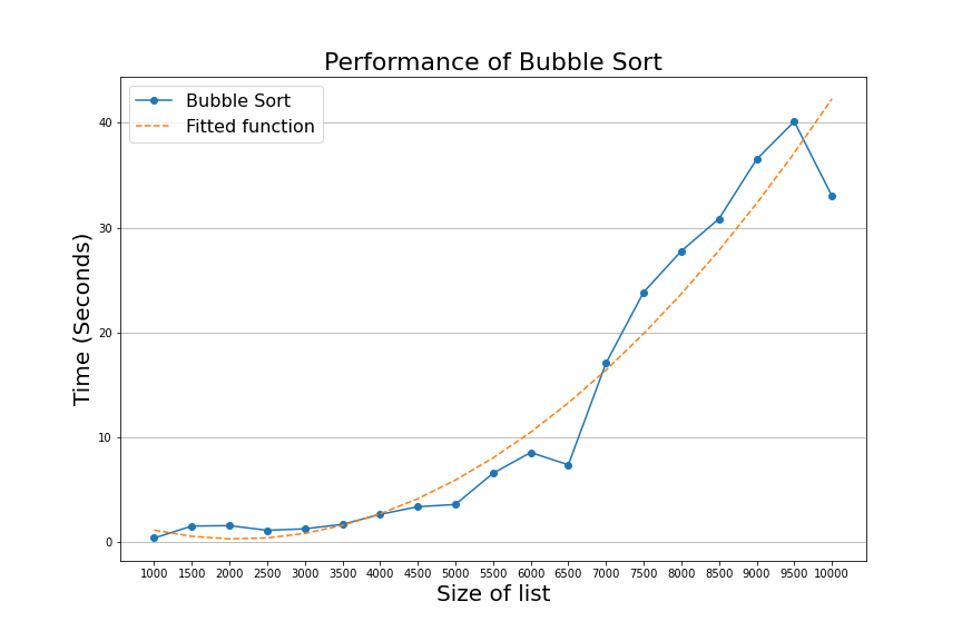
The graph above shows that we can no longer fit a straight line through the algorithm's performance as we did on the get_max_value chart. The performance starts flat at first but begins ramping up as the lists get larger. In this graph, the function \(n^2 \) is a more appropriate description of the algorithm's behavior.

We can see that, just like in the graph of get_max_value, the chart of bubble sort is somewhat erratic and does not follow the fitted function strictly. As we discussed before, this is because the performance of this algorithm is dependent on the machine where bubble sort is executing. This means that we will see different results every time we run this code, but on average, we will see a performance that looks more or less like the graph of  \( n^2 \).

Now that we have executed both algorithms and measured their performance let's compare them in one graph.

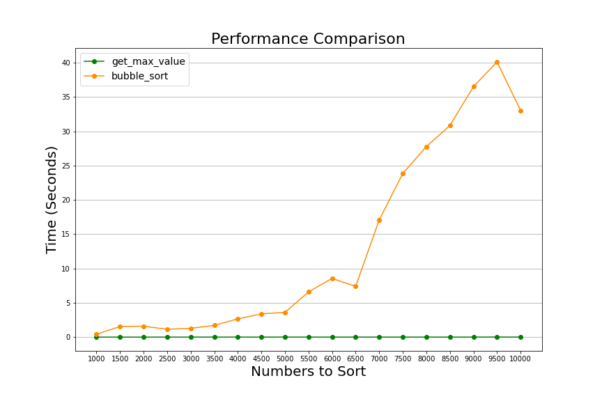
We can now see how bubble_sort performance shoots up compared with get_max_value as the lists grow. By comparison, get_max_value looks like a flat line at the bottom of this graph. The difference in time is dramatic when each algorithm processes the list with ten thousand numbers.

Complexity theory tells us that bubble sort executes ten thousand times more operations when it executes than when finding the maximum value of the same list. In practice, we don't get a ten thousand times increment in time because computers are very good at optimizing operations that execute repeatedly, but it is still a big difference.  

In our experiment, we see that get_max_value takes about .015 seconds to complete, and bubble sort takes around 33 seconds; this is a factor of about 2200 times longer. It is not ten thousand times more, as the theory could make us think, but it is still orders of magnitude longer.

We mentioned previously that this comparison is not fair because these two algorithms' goals are different, and we are not comparing "apples" to "apples." However, our first goal in these two articles was to compare the performance of an \(O(n)\) algorithm with a \( O(n^2) \). Now that we can see the difference firsthand, we can use this as an example for reasoning about algorithms and get a sense of how algorithms behave; this type of reasoning is what helps us make better decisions when writing code.

Conclusion

In this article, we took the theoretical results we got in the previous article and tested them. We ran both get_max_value and bubble_sort with lists of different sizes and measured their execution time. We found that the measurements don't follow the theory strictly. However, we can see that our results follow the theory on average. We also compared the performance of the two algorithms against each other. When we did that, we saw the significant difference in time that an \(O(n^2)\) algorithm has when compared to a \(O(n)\) algorithm as the inputs grow larger.

Finally, we also saw how this comparison is unfair because the get_max_value algorithm is more straightforward than bubble_sort. Each algorithm has different goals, so it is easy to see why bubble sort would take longer. In our next article, we will do an "apples" to "apples" comparison and compare bubble sort with another sorting algorithm and see a better example of how complexity theory can help us make better decisions.