Big-O notation and complexity theory

Big O notation and complexity theory are fundamental concepts in computer science that students typically learn about these topics when they take an algorithms class. Outside academics, Big O notation and complexity theory are mostly buzzwords and occasionally appear during a job interview. In my experience, most people tend to regard these concepts as nothing more than theories that have no place in the real world, but in this article, we will see how these concepts can actually help developers make better decisions when working with code.
This article will look at examples of how to analyze and compare the performance of two algorithms. We will see how understanding these concepts helps developers make more informed decisions that can help in their day-to-day work.
Complexity theory aims to classify algorithms, and big O notation is the notation used to express algorithm categories. This description of big O notation is more or less the definition we find on Wikipedia.
"In computer science, big O notation is used to classify algorithms according to how their run time or space requirements grow as the input size grows."
Classifying an Algorithm
Let's see an example of how an algorithm is classified by its run time. We do this by counting the lines of code an algorithm executes when running.
The function get_max_value above returns the maximum value of an array of numbers. For each line of code, I have written the number of times each line executes when the function runs.
On line 2, we initialize max_value to the minimum possible number; that line only executes once, so we mark that line with a one.
On line 4, we have a loop that goes through every number in the array, so we mark the line as executing an \( n \) number of times.
Lines 5 and 6 will run one time less than line 4 because when the loop ends, it will skip these two lines, so we mark them as running \( n - 1 \) times.
One thing to note here is that line 6 executes at most \( n - 1 \) times. Line 6 runs when the variable num is bigger than max_value, so we will mark the line as \( n - 1 \) because this is the worst-case scenario.
Finally, the return max_value in line 7 will execute one time.
If we add all the steps, we can see that the function's total number of steps is \( 3n \).
In other words, we can say that this function executes three times the number of lines of code as the number of items in the array.
Let's put some real numbers into this calculation.
If the array has ten numbers, we would have thirty steps executed in total, \(3*10 = 30\). If the array has one hundred numbers, we would have three hundred steps in total, \(3 * 100 = 300\).
If we keep going this way, we will have the following table:
| \( n \) | \( 3n \) | Total number of steps |
|---|---|---|
| 100 | 3 * 100 | 300 |
| 1000 | 3 * 1000 | 3000 |
| 10000 | 3 * 10000 | 30000 |
| 100000 | 3 * 100000 | 300000 |
We can see that \( n \) dominates the total number of steps in these calculations. When \( n \) is one thousand, we have a total of three thousand steps, so it is in which is in the order of thousands. If n is ten thousand, then the total is in the order of tens of thousands.
Because \( n \) dominates the calculations, we can simplify our formula and say that the get_max function is in the order of \( n \) because \( n \) dominates the runtime of the algorithm.
Algorithms are classified by finding the function that dominates the execution time. In this case, the get_max_value function is in the order of \( n \), and this is written as \( O(n) \) using big O notation.
I have somewhat oversimplified the processes of classifying an algorithm, but the takeaway here is that once we find the function that dominates the execution in an algorithm, we categorize the algorithm by naming the function that dominates the execution. In this case, we said that the get_max_value algorithm is \( O(n) \).
Visualizing get_max_value
If we plot the number of steps get_max_value takes with inputs of sizes of \( [1,2,3,4,5,6] \) we get the following graph:
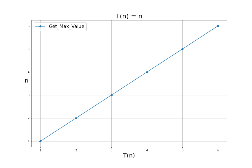
Ok, so at this point, you may be wondering, How can this ever be helpful to developers? Let's be honest; this doesn't look like the type of thing that will help a developer in the next project. This is a valid concern, but bear with me a little longer, and let's look at what else is out there.
We said that the purpose of all this is to classify algorithms. So far, we have seen an algorithm that looks like a line when visualized, but is there anything else we can classify that does not look like a line?
A Non-Linear algorithm
Next, we are going to look at an algorithm called bubble sort.
Bubble sort is a sorting algorithm used to sort lists. For example, the list \( [4,3,5,2,1,6] \) can be sorted by bubble sort, and after being sorted, it will look like this: \( [1,2,3,4,5,6] \).
The bubble sort algorithm does this by comparing each number in the list with every other number, and it exchanges the number's position when they are not in order.
The code for bubble sort is similar to the get_max_value algorithm; the main difference is that it needs an extra loop to compare all the numbers.
Let's analyze the bubble sort code.
On line 2, bubble sort finds the array's length and assigns it to \( n \). This line executes only one time.
On line 4, the algorithm goes through every number in the array; this line will execute \( n \) times.
On line 5, the algorithm will again go through every number starting at zero; this means that in the worst-case scenario, the inner loop will run in full for every iteration of the previous loop, so we will mark this line as executing \( n^2 - 1 \).
Lines 6 and 7 compare and swap the numbers if not in order. We will mark these two lines as executing \( n^2 - 2 \). As we did previously, we subtract two from the total because these lines are under two loops and don't execute when the loops finish.
Line 9 will only execute one time.
Counting the statements in the bubble sort algorithm gives us the following polynomial \( 3n^2 + n - 2 \). We can see that of all these terms, the function that dominates the run time is \( n^2 \).
This makes sense because \( n^2 \) represents the work that happens inside the two loops, and that is where most of the computation will occur; therefore, we can say that bubble sort is in the order of \( O(n^2) \).
We can now compare the get_max_value algorithm with bubble_sort visually in terms of how many steps they take:
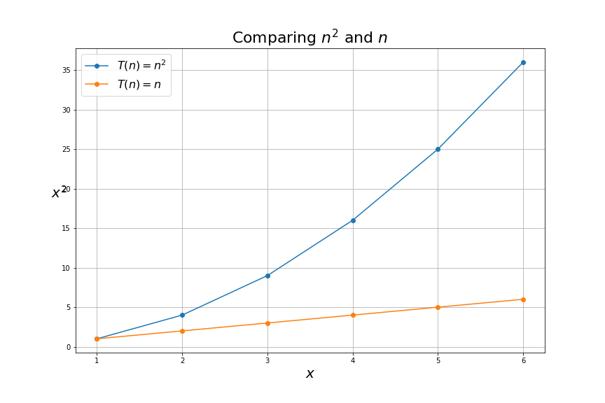
The main takeaway of this graph is that the function \( n^2 \) grows a lot faster than the function of \( n \). This means that the get_max_value algorithm will perform better than bubble_sort because it takes fewer steps.
For example, if \( n \) is 6, get_max_value will take six steps to complete, while bubble sort needs six times more steps. This gets worse as inputs get bigger. If \( n \) is one thousand, get_max_value will take one thousand steps while bubble sort will take one million steps. A thousand times more steps!
Comparing get_max_value and bubble_sort is not really fair because they do different things, and it's easy to see that bubble sort would take longer to complete because sorting a list is more work than finding the maximum number in a list. That being said, comparing the performance of these two algorithms helps us see how algorithms are analyzed.
With this in mind, we can see that if a developer had to choose between two algorithms that accomplished the same goal and one would take \( n \) steps and the other \( n^2 \) steps, the developer would hopefully choose the first option because the computer will take less time in finishing the task.
Applying the theory
Having a description that allows us to categorize algorithms can be very handy when deciding if code will perform well in the real world, but how often is this useful?
One common argument usually heard is that worrying about speed is not a big deal because "computers are very fast nowadays." Computers are indeed faster today than in the past, but we also have a lot more data for computers to process, so it is still very common to encounter performance problems when writing code.
Learning about algorithmic complexity can be a tedious task, and it is easy to think that these concepts are not helpful, but the reality is they are. The good news is we just need the intuition behind the theory. The theory is a tool that teaches us how to build intuition.
This is where Computer Science theory has practical applications. Programmers with intuition for algorithms' performance are better prepared to make good decisions when writing code.
Armed with this intuition, a developer can quickly see that the function with a triple loop that works well in a test environment with one hundred records will not scale well in production, where it will loop through hundreds of thousands of records. This is an extreme scenario, but we can also think about how this can be useful in more subtle cases.
For example, if a developer encounters a function with a double loop and this function works well with one hundred records, then the developer may start asking questions like "How much data will this be processing in production?" "How about in 6 or 12 months?".
It may be that the data is not expected to grow in a production environment, in which case an algorithm with a double loop and a complexity of \( O(n^2) \) will not be a concern. However, if the data is expected to grow into millions of records, the developer needs to start thinking about improving the algorithm.
The answers to these questions can differ depending on the circumstances of each application. Ultimately, it is up to developers to make good decisions about code implementation, and big O notation and complexity theory are tools that can help them make better decisions.
Conclusion
In this article, we saw how we can count the steps of algorithms and how we can build mathematical representations of the number of steps they take. We also saw how these mathematical representations describe the performance of the algorithms by using big-O with a triple loop that works well in a test environment with one hundred records that will not scale well in production, where it will loop, and how we can use big-O notation to compare their performance. We saw that the algorithm for finding the max value is a \(O(n) \) while the bubble sort algorithm has a performance of \( O(n^2) \), and we concluded that \( O(n) \) is better than \( O(n^2) \).
Finally, we talked about how learning this theory can help programmers develop an intuition for writing code that performs efficiently. We saw two very simple examples, but they serve as a starting point for understanding the application of complexity theory. In future articles, we will measure the actual performance of these algorithms to get a better idea of how this theory works in practice.