Comparing sorting algorithms

In the previous article, Measuring the performance of algorithms, we measured the time it took to execute the algorithms bubble sort and get_max_value. That comparison allowed us to see how \(O(n^2)\) algorithms perform compared to an \(O(n)\) algorithm in practice. We saw a big difference in time when we compared the algorithms. However, the algorithms we measured were very different in what they did, so the comparison was unfair.

In this article, we are going to compare two sorting algorithms with different run times but they will both produce the same result. so we are going to see a better example of how complexity theory helps describe the performance of algorithms.

Introducing Merge Sort

Merge sort is a sorting algorithm that relies on a divide-and-conquer strategy. The idea behind merge sort is to take a list of numbers and divide them into the smallest groups possible over the course of multiple iterations, then once divided the numbers get sorted, and finally, all the results are combined to produce the complete sorted list.

The code for merge sort is more complex than that of bubble sort, but it has a better theoretical run time at \(O(nlog(n))\).

The code for merge sort is the following.

Analyzing Merge Sort

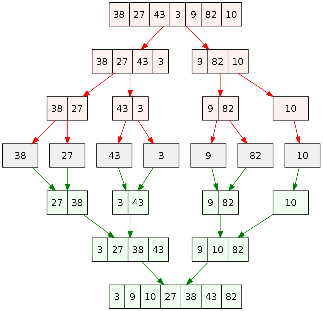
We will analyze merge sort visually since it will be easier to see how this sorting algorithm works instead of counting the number of operations line by line as we did with bubble sort.

As we mentioned previously, merge sort divides the list we want to sort into smaller groups.

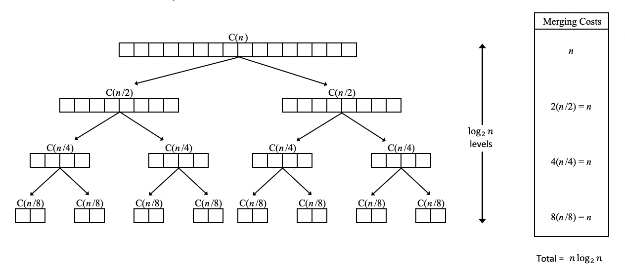
In the picture above, we can see that if we have a list of numbers and divide it into halves until we get to the smallest number of groups possible, it takes a total of \(log_2(n)\) levels of splits. In this case, the list has a size of 16, so if we take \(log_2(16)\) we get 4.

This means we can get to the smallest groups by going through 4 levels of list divisions. Then, we perform an \( n \) number of operations for each level to get each number in the list into the respective group.

The amount of work to divide the list can be represented by \(n * log_2(n) \) operations. Once we have broken down the list into the smallest groups, the next step is to sort the small groups and put the list back together by also sorting each sub-group as the list is put together, which takes an additional \(n*log_2(n)\). But as we saw in the previous analysis, we can take \( n*log_2(n) \) as the description of the performance because this formula dominates the overall execution of the algorithm.

Merge vs. Bubble Sort

let us now measure the time it takes for both sorts to complete, then we will compare their results.

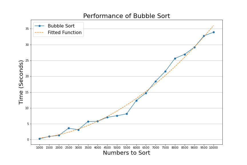
As we saw previously, bubble sort has a performance that has a curve upwards and it looks like the function \(n^2\)

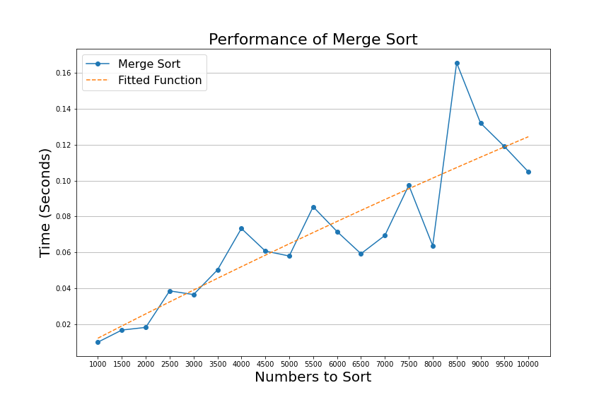
On the other hand, Merge sort has a flatter chart because it follows the function \(n* log_2(n)\).

We can see a significant difference in performance between both sorts from the two charts above. Even though both algorithms are sorting the same lists of numbers, let's look at the results in one chart.

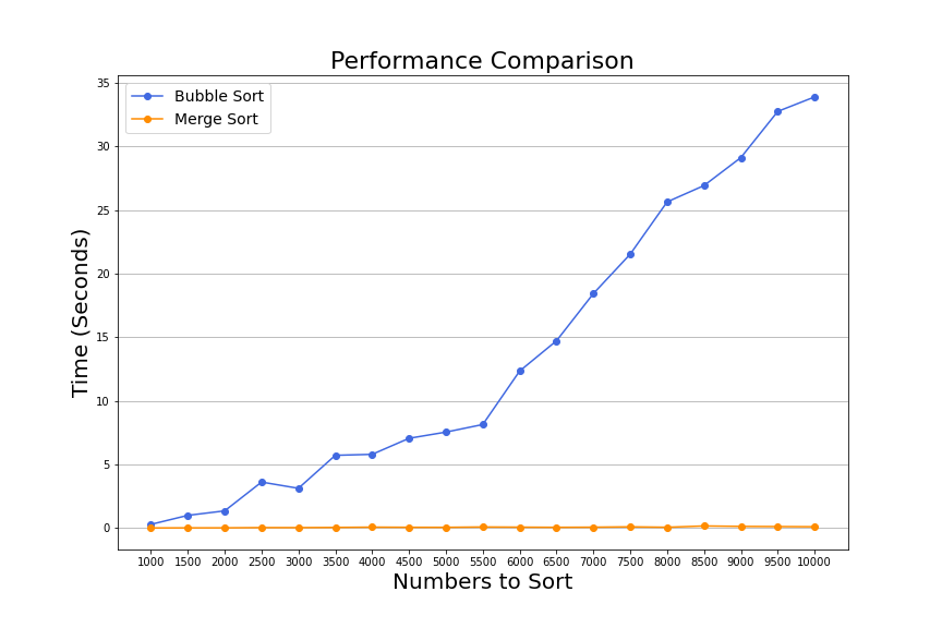
In the graph above, we can see that it took merge sort 0.10 seconds to sort a list of ten thousand numbers. On the other hand, bubble sort took 34 seconds to sort the same list. Merge sort is 340 times faster than bubble sort!

This is an example of the power of algorithms; by being clever, we can speed up the task of sorting a list by a very significant amount. Algorithm analysis can be cumbersome and hard to understand, but the analysis serves as a tool we can use to have a deeper understanding. We can then make better decisions when we have a better understanding of the problem at hand. This is ultimately how developers can benefit from learning to do algorithm analysis.

It is worth mentioning that learning to do algorithm analysis is not the only way to develop the intuition for how algorithms perform. I have met plenty of developers who never learned the formal process of algorithm analysis and can make good decisions when writing code. Algorithm analysis certainly does not preclude writing quality code, but it is a tool that can help.

At the end of the day, there is a connection between what is taught in theoretical classes and what we do in the real world. Many times I have heard students and professionals alike say that what schools teach is useless; I used to think the same, but I have come to realize that this is not the case. It is not that there is a disconnect between computer science theory and the real world. It's just that the connection is not easy to see.

Conclusion

This article visually analyzed the merged sort algorithm and concluded that it is an \(nlog_2(n)\) algorithm. We also saw that it is a more complex algorithm when compared to bubble sort, but it is a much more efficient algorithm. Next, we took merge sort for a test drive, measured the performance on ten lists ranging from one thousand to ten thousand items, and then compared the results with the results we got from bubble sort. We saw that merge sort gave us a better performance as the list grew in size.

We have been building a bit of the background necessary for algorithms analysis in this series of articles. However, comparing sorting algorithms still feels "too academic," so in our next article, we will look at a real-world example of when choosing the correct algorithm can make a big difference in the world of PC gaming.